How many times you wake up one morning and see the reward of your efforts waiting for you to be opened. Happens with me quite often to me.
However this one is special as this time the reward was for something I fell in love around 10 years ago and in the past 5 years I don’t think I did justice to my love. The reward for my interest in Mathematics, one of the most beautiful art someone can learning. And learning to think like a real mathematician is even tougher. And I can go on and on about the joys and benefits of learning and practicing the art of mathematics.
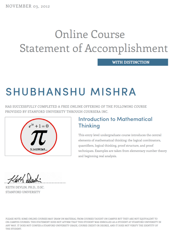
However long story cut short. The reward which I got when I woke up and opened my mail box was, a certificate of course completion with distinction for Introduction to Mathematical Thinking by Keith Devlin on Coursera. The course was run from September 17th, 2012 for 7 weeks and constituted of video lectures on elementary mathematical logical topics like operators, logical quantifies and combinators, methods and languages of mathematical proofs and yes number theory, set theory and real analysis.
There were a lot of important features of the course which I really liked:
- The instructor: Yes I am talking about Prof. Keith Devlin, he is a wonderful professor who not only taught the course, but he also took us on the journey of exploration in the world of mathematics, some of the anecdotes which he quoted at various points during his videos made the course watching a lot more fun.
- The lecture videos: The lecture videos though at times long like class lectures were prepared in an absolutely engaging and thought provoking manner. Prof. Devlin took one topic at a time and took us through the various ways of dealing with the problem. Of great interest is his video on Implication operator where he explained very slowly and precisely what the operator does. The lecture videos were very well supported with in video quizzes which were a great way to be engaged in the video rather than just watch it and doze off.
- The quizzes and assignments: The assignments and quizzes were very directly related to the course material and involved that we are learning the basic thing about the course i.e. to think like a mathematician, reasoning out our solutions becoming sure of it. It was aimed more towards learning how to reason and use logic than to just find the solution.
- The peer assessment system: This was actually the most favorite part of the course and also the one through which I felt learnt the most. The peer review process is very different from one professor checking all the answers or utilizing an MCQ for easier grading. When the answers require mathematical thinking and there are infinite ways [ I think we can take that proving exercise] of proving the same thing, the above mentioned grading methods fail. In this scenario the peer grading system works very well and not only we get a chance to assess our fellow course takers but we also get to know some of the other beautiful ways of working out the same problem. I really liked the solution of some of my fellow test takers during the final exam and many times it gave me immense pleasure to see how my answer was the way some of the other people have solved the same problem.
- Engaging articles shared during the course: Prof. Devlin made sure that he is not just giving us academic material but also other interesting ways of learning the application of course. He kept writing a blog [http://mooctalk.org/] on his experience of teaching the course. He also shared with us things he thought might make learning mathematics more interesting for us.
- The certificate of course completion: I was happy that I could finish the course with distinction. I never thought it would be possible for me as I was taking the course while commuting back from office in my cab every day and used to do problems at home. The 1st peer assessment assignment and the final exam was the time I got really serious about completing the course professionally. So I was happy that I made it among the top students who completed the course. By the way, here is the certificate.
I have studied these courses in college and was deeply demotivated at the teaching style which made me cut off from mathematics which was a part of our curriculum. However, I always wished to take a really interesting course like this to get back to mathematics. So I was really excited when I heard of this course on coursera. I like the platform a lot and I feel its a great way for people to learn new subjects from interesting and knowledgeable professors from around the world.
The major things I learned from the course were:
- Mathematical Thinking: I feel its very important to approach a problem in mathematical way rather than to just find its solution. The difference is that at every step you have to justify your approach and the reasons you are giving. The idea is to be completely precise with your language and facts. Mathematical language looks tough but is fairly simply to comprehend once you get hold of it. The absence of ambiguity in a perfectly crafted mathematical statement, not only makes it more significant but also tried to bring its beauty to the maximum. This by far I feel is the biggest learning from the course.
 : I always wanted to learn
  but never felt a requirement to implement it and sometimes I was just too lazy. I loved reading the latex publications and the beautiful mathematical equations which are impossible to replicate in a word processor. Learning latex was fun as I tried using it for my peer assessment solutions. I wrote all solutions in latex and once because of time limit even missed answering 2 sub sections in a question because of deadline. I know how to write mathematical statements in now and would be learning it to write publications as well.
- Peer Assessment and Grading Rubric: I feel this has been another great learning from the course. I liked the process of peer reviewing as it initially forced me to look carefully at the solutions of others which I later enjoyed. I liked looking at the mathematical reasoning presented. Some of the students just gave flawless bulletproof solutions which were a delight to read. Some were sloppily written so I felt a bit disappointed but I learned a new of how not to answer that question.
- Take time while working out a solution: Prof. Devlin mentioned this in his first video lecture and the idea looked very correct. The joy of solving a problem without worrying about finding a solution in time is amazing. You can look at ways which will not work, you will find ways which can work for other solutions but not this one, in the process broadening your understanding of the subject.
There were a few regrets I had though .Because of my office hours and other engagements I was not able to follow the timeline of the course so sometimes I will just go through all videos in one day. I focused mainly on solving problems which I could do without a computer. Another regret was being unable to utilize the power of the community which I only got to know during the peer assessments. I feel these things were also a very important element of the course journey and I wish to follow them in my future courses on a MOOC.
Overall I would suggest this course to all individuals interested in mathematics and try to enjoy the journey to the fullest. Try to utilize the community to the maximum and enjoy solving the assignments. In the end I leave this with the most beautiful equation in mathematics which was also used as the logo for the course.


 .
.
You must be logged in to post a comment.